If you are one of the companions of Abaqus training and practical examples section on the reference site for training mechanical software, you have become familiar with the importance and wide application of mechanical connections. Previously, in a series of educational examples, we have examined the weld (from the stress and thermal point of view) and the screw (from the stress point of view) as two common industrial connections (here: Modeling and analysis of T-shaped welds in Abaqus – Heat transfer analysis in the process Welding by Abaqus software – analysis of threaded joints by Abaqus).

 

The field of industrial connections can be considered as one of the difficult issues in finite element analysis. Due to the sudden contact between two pieces and the change of the geometry of the pieces during the process of fitting and connecting, the convergence of the solutions is difficult in solving by software such as Abaqus. Therefore, it is possible to recommend the use of Explicit solvers in this category of problems as a path-breaking tool. Do not forget that using the Explicit solution method does not guarantee the correctness of the results. In this example, you will learn to simulate and analyze the process of fitting two connecting pieces together with the help of an Explicit solver, so follow the solution steps carefully.

The solution of the problem of the analysis of the plug connection in Abaqus

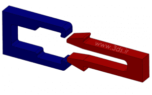
We intend to establish a connection between the two parts below by creating a horizontal force and through the process of cutting. Analyze the process with an Explicit solver in Abaqus and draw a graph of the force created between the two pieces in terms of time.

Note: Download the model file of this project in Solidorex (file format in the attached file).

Solving the problem of joint analysis by Abaqus

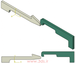
As we have mentioned many times, reducing the solution time in finite element analysis is one of the vital and important points. Therefore, due to the existence of geometric symmetries and loading in this problem, we will use the model of a quarter of parts for simulation in Abaqus. Therefore, after downloading the relevant file, go to File → Import → Part to call the desired geometry in Abaqus.

In the second step of the solution, enter the Property module and define a material with the following mechanical properties:

Young’s modulus: 3GPa, Poisson’s ratio: 0.4 and density 3ton/mm3

Then define two homogenous Solid sections and assign them to both existing pieces for analysis. Next, enter the Assembly module and place the parts according to the image below. If you have used the mentioned file, there is no need to make any changes.

According to the nature of the problem (loading and unloading), in the Step module, create two solution steps of the type Dynamic, Explicit and with a time interval of 0.1s. Accept other Abaqus defaults in this module and enter the Interaction environment.

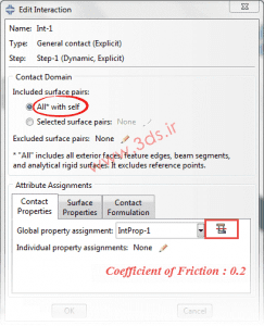
In this section, define a General type contact with a friction coefficient of 0.2 as shown in the image below.

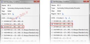
Then enter the Load module and in the first step, apply the symmetries related to the Z and Y axes in both parts.

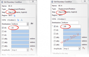
Next, bind the big piece in the X direction and move the smaller piece 15 units to the right in the first step and change the amount of displacement to -15 in the second step.

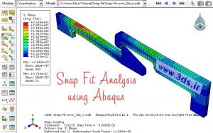
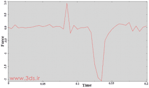
In the last step of modeling the problem, go to the Mesh module and mesh both parts with a mesh of 0.75 grain size. Then send the problem to the Job module to solve it. The diagram below shows that the amount of force required to insert the parts is about half of the force required to pull the parts out from each other.

The following animation shows the tension contour of the assembly during the above process.